Spectral Endmember Extraction: The Spectral Hourglass Workflow
Or: How to Find Pure Pixels in a Mixed-Up World
Introduction: What Are Endmembers Anyway?
In hyperspectral remote sensing, each pixel’s spectrum represents a mixture of pure materials called endmembers. Think of it like a smoothie - you can taste the banana, strawberry, and yogurt separately, but they’re all blended together.
Key concept: Every spectrum in an image can be reconstructed as a combination of endmember spectra. The theoretical maximum number equals the number of bands plus one (representing the composite background).
The Spectral Hourglass Workflow
The spectral hourglass systematically reduces data dimensionality while extracting the purest spectral signatures. This proven methodology supports applications in mineral exploration, vegetation analysis, and environmental monitoring.
Sequential steps:
- Reflectance Data - Atmospherically corrected imagery
- MNF Transform - Dimensionality reduction and noise separation
- PPI Calculation - Pure pixel identification
- N-D Visualizer - Interactive endmember extraction
- Spectral Mapping - Material abundance calculation
Step 1: Minimum Noise Fraction Transform
MNF separates coherent signal from random noise through two-stage principal components analysis. This critical preprocessing enables effective endmember extraction.
How MNF Works
Stage 1: Noise Estimation - Shift-difference method calculates local pixel variance - Produces noise covariance matrix
Stage 2: Transformation - First PC transform decorrelates and rescales noise - Second PC transform on noise-whitened data - Bands ranked by decreasing eigenvalues
Determining Spatial Coherence
Signal bands: - High eigenvalues (> 1.0) - Visible spatial structure - Coherent image features
Noise bands: - Eigenvalues approaching 1.0 - Random spatial patterns - No recognizable features
Best practice: Include all MNF bands with eigenvalues above unity. Typical retention: 10-30 bands.
Step 2: Pixel Purity Index Algorithm
PPI identifies spectrally pure pixels by projecting data onto random vectors through n-dimensional space.
PPI Methodology
The algorithm: 1. Generates random vectors through data cloud centroid 2. Projects pixels onto each vector 3. Marks extreme positions as “pure” 4. Repeats thousands of times (10,000-50,000) 5. Accumulates purity scores
PPI Results
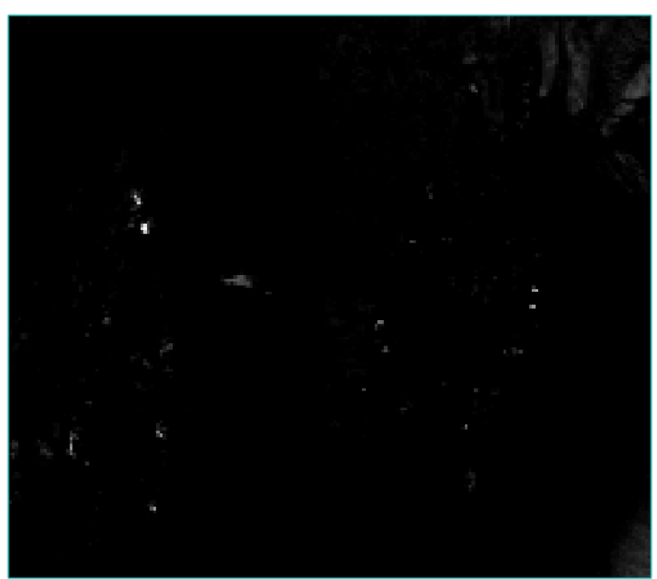
Output characteristics: - Pixel values = detection frequency - Bright pixels = high purity (data cloud corners) - Most pixels score near zero - High-scoring pixels input to N-D Visualizer
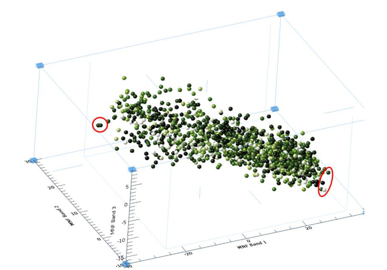
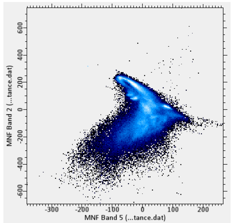
Step 3: N-Dimensional Visualization
The N-D Visualizer enables interactive exploration of spectral space to locate and extract endmembers.
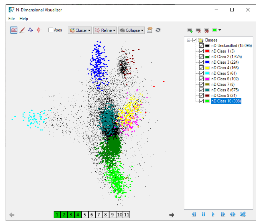
Understanding N-Dimensional Space
Geometry: - N dimensions = number of MNF bands - Each band = one orthogonal axis - Pixel spectral values = coordinates - Data forms irregular volumetric cloud
Convex hull principle: Pure endmembers always occupy vertices of the convex hull. Cloud corners contain pure pixels, interior contains mixed pixels.
Interactive Selection
Extraction process:
- Rotate data cloud through all MNF dimensions
- Identify protruding pixel clusters at corners
- Draw selection regions around clusters
- Assign unique colors to each endmember class
- Export endmembers to spectral libraries
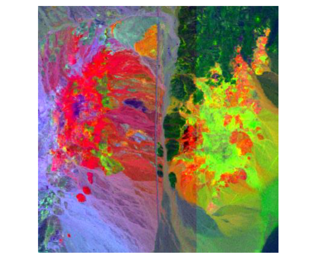
Spectral Mapping Methods
After endmember extraction, multiple methods enable material mapping and abundance estimation.
Method Comparison
| Method | Type | Input | Output |
|---|---|---|---|
| SAM | Similarity | Reflectance | Classification |
| SFF | Feature | Reflectance | Probability |
| Linear Unmixing | Complete | All endmembers | Abundance % |
| MTMF | Partial | Target endmembers | Abundance + feasibility |
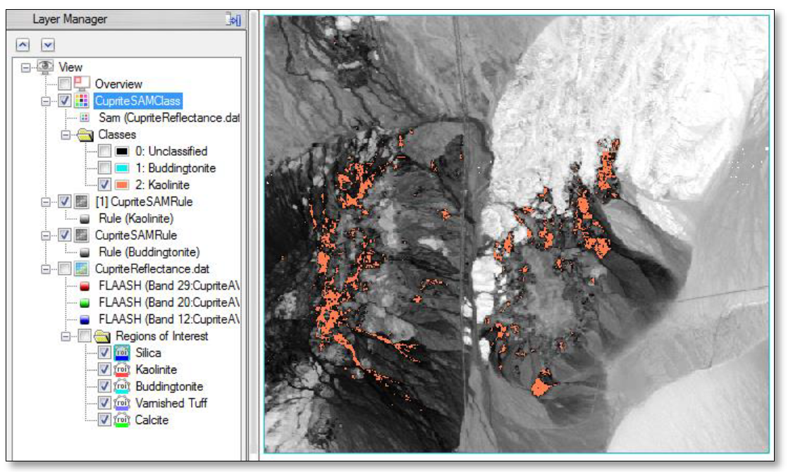
Spectral Angle Mapper (SAM)
Measures spectral similarity via n-dimensional angle. Smaller angles = closer matches. Produces classification maps assigning each pixel to best-matching endmember.
Linear Spectral Unmixing
Estimates sub-pixel abundances assuming linear mixing of endmembers. Requires all scene endmembers identified. Outputs abundance images showing 0-100% coverage per endmember.
Best Practices Guide
MNF Parameters
- Use all bands with eigenvalues > 1.0
- Typical retention: 10-30 bands
- Overestimate rather than underestimate
PPI Parameters
- Minimum 10,000 iterations
- 20,000-30,000 for moderate complexity
- 50,000+ for heterogeneous scenes
- Monitor cumulative plot for leveling
Endmember Count
- 10-20 endmembers typical
- More for heterogeneous scenes
- Balance detail against noise
Validation
- Compare with field spectra
- Verify spectral uniqueness
- Check spatial distribution
- Cross-reference ancillary data
Conclusion
Spectral endmember extraction forms the foundation of quantitative hyperspectral analysis. The spectral hourglass workflow—MNF transformation, PPI calculation, and N-D Visualizer selection—enables reliable extraction of pure spectral signatures for material mapping across diverse applications.
Contact
Email: mapcrafty@gmail.com
Subject: “Spectral Endmember Extraction Consultation”