Monitoring Vegetation Health with Google Earth Engine: A Complete NDVI Analysis Tutorial
Introduction
Vegetation monitoring is crucial for agriculture, environmental conservation, and climate research. In this tutorial, we’ll walk through a complete Google Earth Engine (GEE) workflow that analyzes vegetation health using NDVI (Normalized Difference Vegetation Index) from Sentinel-2 satellite imagery over a 6-month period in Germany.
What you’ll learn: - How to filter and process Sentinel-2 imagery - Calculate NDVI for vegetation analysis - Automate bulk exports to Google Drive - Visualize results on an interactive map
Understanding the Code: Step by Step
1. Setting Up the Time Range
var endDate = ee.Date(Date.now());
var startDate = endDate.advance(-6, 'month');
print('Start Date:', startDate);
print('End Date:', endDate);
What’s happening here: This section establishes our temporal window for analysis. We’re creating a 6-month period ending today: - ee.Date(Date.now()) captures the current date - advance(-6, 'month') moves backward 6 months from today - The print() statements display these dates in the Console for verification
Why 6 months? This timeframe captures seasonal variations in vegetation while keeping the dataset manageable.
2. Loading Sentinel-2 Imagery
var s2 = ee.ImageCollection('COPERNICUS/S2_SR_HARMONIZED')
  .filterBounds(aoi)
  .filterDate(startDate, endDate)
  .filter(ee.Filter.lt('CLOUDY_PIXEL_PERCENTAGE', 20));
print('Total images available:', s2.size());
Breaking it down: - 'COPERNICUS/S2_SR_HARMONIZED' - This is the Sentinel-2 Surface Reflectance collection, atmospherically corrected and ready for analysis - .filterBounds(aoi) - Filters images to only those intersecting our Area of Interest (AOI) in Germany - .filterDate(startDate, endDate) - Limits images to our 6-month window - .filter(ee.Filter.lt('CLOUDY_PIXEL_PERCENTAGE', 20)) - Critical filter: Only keeps images with less than 20% cloud cover to ensure quality data
Why Surface Reflectance? SR data is already atmospherically corrected, making it suitable for time-series analysis and vegetation indices.
3. Calculating NDVI
function addNDVI(image) {
  var ndvi = image.normalizedDifference(['B8', 'B4']).rename('NDVI');
  return image.addBands(ndvi)
    .copyProperties(image, ['system:time_start', 'system:index']);
}

var s2WithNDVI = s2.map(addNDVI);
Understanding NDVI: NDVI (Normalized Difference Vegetation Index) measures vegetation health using this formula:
NDVI = (NIR - Red) / (NIR + Red)
In Sentinel-2: - B8 = Near-Infrared band (NIR) - strongly reflected by healthy vegetation - B4 = Red band - absorbed by vegetation for photosynthesis
The function explained: 1. normalizedDifference(['B8', 'B4']) - Automatically calculates (B8-B4)/(B8+B4) 2. .rename('NDVI') - Names the new band for easy reference 3. .addBands(ndvi) - Adds NDVI as a new band to the original image 4. .copyProperties() - Preserves timestamp and metadata (essential for time-series)
NDVI Values interpretation: - -1 to 0: Water, bare soil, snow - 0 to 0.3: Sparse vegetation, stressed plants - 0.3 to 0.6: Moderate vegetation - 0.6 to 1: Dense, healthy vegetation
4. Automated Monthly Export Function
function getTwoImagesPerMonth() {
  for (var m = 0; m < 6; m++) {
    var monthStart = startDate.advance(m, 'month');
    var monthEnd = monthStart.advance(1, 'month');

    var monthImages = s2WithNDVI
      .filterDate(monthStart, monthEnd)
      .sort('CLOUDY_PIXEL_PERCENTAGE')
      .limit(2);
The strategy: This function intelligently selects the two clearest images per month over 6 months (up to 12 images total):
- Loop through 6 months (
for (var m = 0; m < 6; m++)) - Define monthly boundaries for each iteration
- Filter images to that specific month
- Sort by cloud cover - clearest images first
- Limit to 2 images - balances temporal coverage with data volume
Why 2 images per month? This captures early and late-month conditions while avoiding data overload.
5. Export Configuration
var imageList = monthImages.toList(2);
var count = monthImages.size().getInfo();

print('Month ' + m + ': Found ' + count + ' images');

for (var i = 0; i < count; i++) {
  var img = ee.Image(imageList.get(i));
  var ndvi = img.select('NDVI').clip(aoi);

  var date = ee.Date(img.get('system:time_start'));
  var filename = ee.String('ndvi_aoi_germany_').cat(date.format('YYYY_MM_dd'));
Export preparation: - Converts the ImageCollection to a list for iteration - Gets the actual count of available images (might be less than 2) - Extracts only the NDVI band (not the full multi-band image) - Clips to AOI boundaries to reduce file size - Creates descriptive filenames with dates (e.g., ndvi_aoi_germany_2024_04_15)
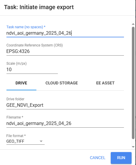
6. Google Drive Export Tasks
Export.image.toDrive({
  image: ndvi,
  description: filename.getInfo(),
  folder: 'GEE_NDVI_Export',
  fileNamePrefix: filename.getInfo(),
  region: aoi,
  scale: 10,
  crs: 'EPSG:4326',
  maxPixels: 1e13,
  fileFormat: 'GeoTIFF'
});
Export parameters explained: - folder: 'GEE_NDVI_Export' - Creates/uses this folder in your Google Drive - scale: 10 - 10-meter resolution (Sentinel-2’s native resolution for visible/NIR bands) - crs: 'EPSG:4326' - WGS84 coordinate system (standard lat/lon) - maxPixels: 1e13 - Allows large exports (10 trillion pixels) - fileFormat: 'GeoTIFF' - Compatible with QGIS, ArcGIS, Python (rasterio), R
Important: These export tasks are queued, not executed. You must manually run them from the Tasks tab.
7. Map Visualization
var ndviVis = {
min: -1,
max: 1,
palette: ['blue', 'white', 'green']
};
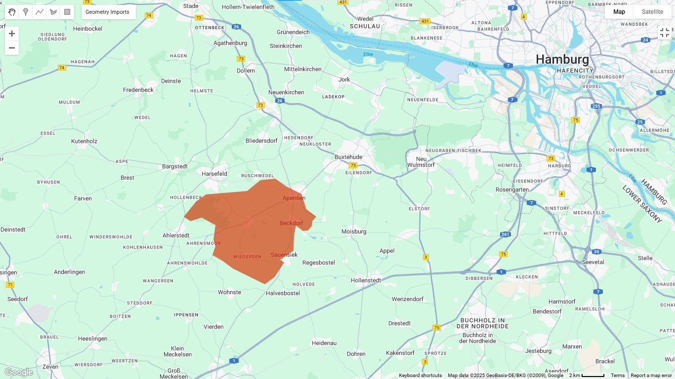
Map.centerObject(aoi, 10);
Map.addLayer(aoi, {color: 'red'}, 'AOI');
var recentNDVI = s2WithNDVI
.sort('system:time_start', false)
.first()
.select('NDVI')
.clip(aoi);
Map.addLayer(recentNDVI, ndviVis, 'Most Recent NDVI');Visualization setup: 1. Color palette: Blue (water/bare soil) → White (sparse vegetation) → Green (dense vegetation) 2. Center map on the AOI at zoom level 10 3. Display AOI boundary in red for reference 4. Show most recent NDVI - uses .sort('system:time_start', false) to get the latest image
Visual interpretation: When you run this code, you’ll see your AOI with vegetation displayed in green tones. Darker green indicates healthier, denser vegetation.
Practical Applications
This workflow can be adapted for:
Agriculture - Monitor crop growth stages - Detect irrigation issues - Assess drought stress
Forestry - Track deforestation - Monitor forest health - Assess wildfire recovery
Environmental Science - Study seasonal phenology - Assess wetland conditions - Monitor urban green spaces
Climate Research - Analyze vegetation response to climate events - Study land cover changes - Track ecosystem productivity
Tips for Success
- Define your AOI carefully - Use the geometry tools in GEE or import a shapefile
- Check the Console output - Verify you have enough images before exporting
- Adjust cloud threshold - If you get too few images, increase from 20% to 30%
- Monitor export limits - Google Earth Engine has daily export quotas
- Batch process exports - Run 3-4 tasks at a time to avoid timeouts
Next Steps
Once you have your NDVI GeoTIFFs exported, you can:
- Time-series analysis in Python using
rasterioandpandas - Create animations showing vegetation changes over time
- Statistical analysis comparing different months or years
- Machine learning for crop classification or anomaly detection
Conclusion
This Google Earth Engine workflow demonstrates the power of cloud-based Earth observation. With just a few dozen lines of code, you can process terabytes of satellite data, calculate vegetation indices, and export ready-to-analyze datasets—all without downloading raw imagery or managing local storage.
The beauty of GEE is its scalability: this same code works whether your AOI is 1 km² or 10,000 km². Just adjust the maxPixels parameter and let Google’s infrastructure handle the heavy lifting.
Ready to try it yourself? Head to Google Earth Engine Code Editor and start exploring!
Resources
📧 Contact & Collaboration
Have questions about this analysis or interested in collaborating on geospatial projects? We’d love to hear from you!
Get in touch with our research team: - Email: mapcrafty@gmail.com - Subject line: “Inquiry about Remote Sensing Applications for air quality Monitoring”
Whether you’re working on similar research, need technical consultation, or want to discuss potential collaborations in geospatial analysis, don’t hesitate to reach out. Our team is always excited to connect with fellow researchers and practitioners in the GIS and remote sensing community.
We typically respond within 24-48 hours and welcome discussions about methodology, data sources, and potential research partnerships.